Annual distributions from the endowment are a source of supplemental operating revenue for most endowed institutions. An institution’s endowment spending policy provides a basis for the calculation of the annual distribution, serving as a bridge that links the long-term investment portfolio (LTIP) and the enterprise. Spending policies are designed to reflect the needs of current and future generations of stakeholders, balancing the goals of providing appropriate levels of support to current operations and preserving, or even growing, endowment purchasing power.[1]Purchasing power is defined as the real market value of the endowment. An endowment that is maintaining purchasing power is keeping pace with inflation (after spending and investment returns). An … Continue reading
The data and analysis in this report cover a variety of spending topics including spending rule types, the endowment’s support of operations, and effective spending rates. This year’s report also examines the concept of intergenerational equity and what that entails with respect to the endowment’s market value and spending distributions. The Cambridge Associates Endowment Spending Model is used to analyze spending scenarios in both a high return and low return environment and the effects those environments have on intergenerational equity.
Participants and Spending Rule Types Defined
For 2015, Cambridge Associates collected spending policy data for 272 of our nonprofit clients, including 154 colleges and universities, 42 cultural and environmental institutions, 25 independent schools, 18 health care organizations, and 33 other nonprofit institutions. Foundations were excluded from the survey group as their spending is influenced by certain spending requirements mandated by the government. A list of participants can be found at the back of the report. Figure 1 shows the distribution of these institutions across various asset size bands.

Figure 1. Profile of Participating Institutions
Source: Spending policy data as reported to Cambridge Associates LLC.
Institutions in this study use three primary spending rule types. Market value–based rules link the spending amount directly to the endowment’s market value. Constant growth rules increase spending each year by a defined growth factor. Hybrid policies combine the elements of both market value–based and constant growth rule types.
Figure 2 shows the prevalence of the spending rule types across participating institutions. The most frequently used rule type is a market value–based policy, cited by 76% of institutions. Market value–based rules are most common among the smallest portfolios, with nearly 90% of institutions with assets under $200 million using this rule type. In comparison, 59% of institutions with assets over $1 billion use a market value–based rule. Hybrid and constant growth rules were cited by 10% and 9% of all participants, respectively. Both rule types were more likely to be used by larger portfolios than smaller portfolios. Among the institutions with assets over $1 billion, 20% used a hybrid policy and 15% used a constant growth policy.
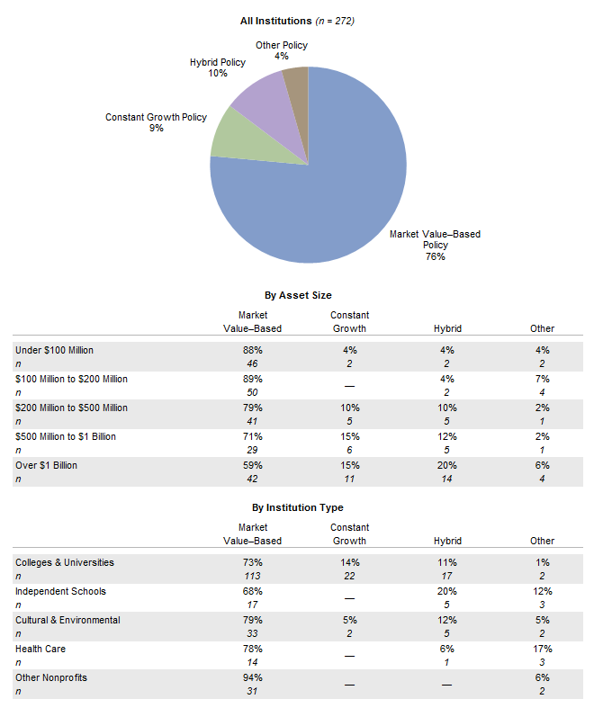
Figure 2. Spending Policy Types
2015
Source: Spending policy data as reported to Cambridge Associates LLC.
Notes: Market value–based spending policies base spending on a prespecified percentage of a moving average of market values. Constant growth policies increase prior year’s spending by a measure of inflation and/or a prespecified percentage. Hybrid policies are those that incorporate a weighted average of a constant growth rule and a percentage of market value rule. Other policies are those that cannot be classified as market value–based, constant growth, or hybrid policies.
Figure 3 shows the distribution of rule types for the 160 institutions that provided spending policy data in 2010 and 2015. The market value–based rule continues to be the most common among institutions in this study. Compared to 2010, two fewer institutions used a market value–based policy in 2015, four more institutions used a hybrid policy, and two fewer institutions used some other policy. The same number of institutions used a constant growth policy in 2010 and 2015.

Figure 3. Spending Policy Types: 2010 vs 2015
Source: Spending policy data as reported to Cambridge Associates LLC.
Note: Bar graph represents the 160 institutions that provided a spending policy in both 2010 and 2015.
Market Value–Based Rules
A market value–based rule dictates spending a percentage of a moving average of endowment market values. By linking the spending distribution amount directly to the endowment’s market value, this rule type usually produces the most dramatic changes in spending when investment conditions shift. Therefore, purchasing power preservation is prioritized during periods when the endowment’s market value declines.
The primary levers of this rule type are the target spending rate and the date or smoothing period used to measure the market value. Some institutions also use a cap and floor to contain changes in the annual spending distribution during volatile market periods.
Target Spending Rate. The target spending rate helps determine the proportion of the endowment that is distributed on an annual basis. Institutions incorporate long-term investment return expectations and inflation into the selection of the appropriate target spending rate. To preserve the purchasing power of an endowment,[2]In this instance, we use the term “endowment” to refer to a single fund with no future inflows. A long-term investment pool, which is a collection of multiple endowments and other long-term … Continue reading the spending rate would align with long-term real investment return expectations. The purchasing power of an endowment will increase when the spending rate is lower than the long-term real return, and vice versa.
In 2015, most participating institutions that cited a market value–based rule used a pre-specified target rate (88%), while the remaining institutions allowed some discretion by setting a pre-specified percentage range within which the target spending rate may fall. For the purposes of comparing target spending rates, we assume the midpoint for institutions that specified a discretionary range. Of institutions with a market value–based policy, 48% used a target spending rate of 5%, while 41% of respondents used a target rate below 5%. Only 11% of institutions applied a rate that exceeded 5% (Figure 4).

Figure 4. Characteristics of Market Value–Based Spending Policies
2015
Source: Spending policy data as reported to Cambridge Associates LLC.
Notes: Market value–based spending policies base spending on a prespecified percentage of a moving average of market values. Graph reflects data for the 206 institutions that provided detailed data on their target spending rate. If a range was provided, the target spending rate was calculated using the midpoint of the range.
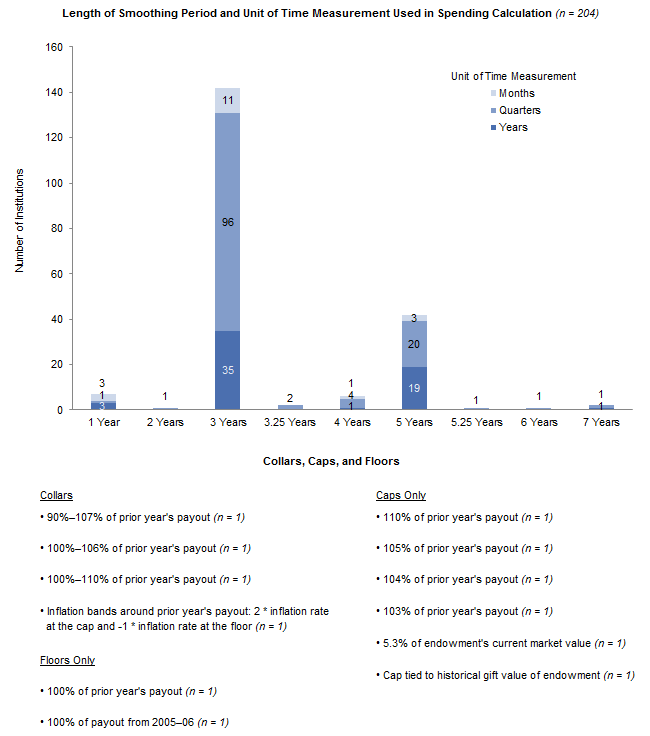
Figure 4 (continued). Characteristics of Market Value–Based Spending Policies
2015
Source: Spending policy data as reported to Cambridge Associates LLC.
Notes: Market value–based spending policies base spending on a prespecified percentage of a moving average of market values. Unit of time measurement indicates whether spending is calculated using monthly, quarterly, or yearly market values. Graph reflects data for the 204 institutions using a market value–based spending policy that provided the unit of time measurement in their spending calculation.
Over 70% of institutions reporting data since 2010 have made no change to their target spending rate. Of the remaining institutions, 19% indicated a decrease in their rate when comparing 2010 and 2015 (Figure 5). The decreases ranged from 0.1 ppt to 1.0 ppt. For the 10% of institutions that raised their target spending rate over the five-year period, increases ranged from 0.03 ppt to 2.13 ppts.
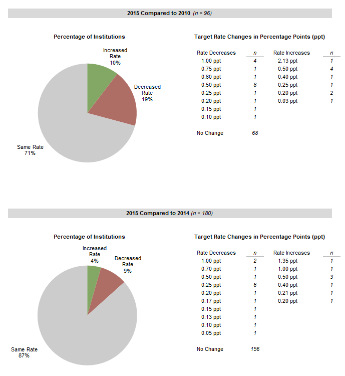
Figure 5. Changes in Target Spending Rates for Market Value–Based Spending Policies
2015 vs 2010 and 2014
Source: Spending policy data as reported to Cambridge Associates LLC.
Notes: Market value–based spending policies base spending on a prespecified percentage of a moving average of market values. Graphs reflect data for the institutions using a market value–based spending policy that provided the target rate used in their spending calculation for fiscal year 2010 or 2014. If a range was provided, the target spending rate was calculated using the midpoint of the range.
Smoothing Period. The spending distribution under a market value–based rule is determined by applying the target spending rate to the endowment’s market value. This is usually measured as an average market value over a period of time, known as a smoothing period. By capturing the endowment’s market value over several points in time, the smoothing period helps reduce the year-to-year volatility in spending distributions. Smoothing periods for participants in this report range from one to seven years, and the time interval (i.e., monthly, quarterly, or annual market values) can vary (Figure 4). The most common measurement period was 12 quarters (47% of those with a market value–based policy).
Cap and Floor. The introduction of a spending floor and/or cap can also serve as a smoothing mechanism for spending dollars by limiting the change in spending during particularly volatile periods. In a market value–based rule, a floor prevents spending from falling below a certain level, usually the previous year’s spending dollar amount. While a floor can relieve budgetary pressures during market downturns for institutions with concerns about spending cuts, limiting the decline in distributions can further erode the endowment’s market value and make purchasing power preservation more challenging over the long run. A cap limits spending increases when endowment growth is particularly strong by setting a maximum annual growth rate. When paired together, a cap and floor (known as a collar) can produce smoother distributions by maintaining a level of spending during challenging economic environments and saving a greater portion of investment gains from periods with exceptional endowment growth.
In practice, only 12 institutions (6%) that use a market value–based rule employ a cap and/or floor. Ten institutions use a cap and/or floor based on a percentage of a prior year’s spending distribution, while one institution applies a cap to the endowment’s market value on a specific date. Another institution links its cap to the historical gift value of the endowment. For the 24 institutions that outline a discretionary range for the target spending rate, the range serves as a collar in that it allows institutions to raise the rate of spending in down markets and lower the rate of spending when endowment growth rates are high.
Constant Growth Policies
A constant growth spending policy increases the prior year’s spending amount by a measure of inflation and/or a pre-specified percentage. Institutions tend to use this rule type when the endowment is a significant source of operating revenue and volatility in annual spending distributions is less tolerable. More predictable spending is derived from constant growth rules with a fixed annual increase in spending rather than those linked to inflation, which is not a constant number and not known in advance. Of the 24 institutions that use this rule type, 12 use a pre-specified percentage growth rate; nine use an inflation-index growth rate; and three use an inflation-index growth rate plus a pre-specified percentage (Figure 6).
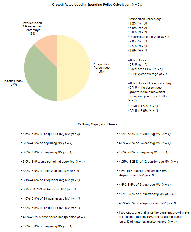
Figure 6. Characteristics of Constant Growth Spending Policies
2015
Source: Spending policy data as reported to Cambridge Associates LLC.
Note: Constant growth policies increase prior year’s spending by a measure of inflation and/or a prespecified percentage.
While the strict application of a constant growth rule produces predictable spending, this rule type has some notable shortcomings. Increasing spending during prolonged periods of low or negative investment returns quickly eats away at an already dwindling market value and may permanently impair the endowment. Figure 7 illustrates this effect using the trailing 15-year period ending June 30, 2015, over which a simple portfolio consisting of 70% equities and 30% bonds produced a real return of just 3.2%.[3]Returns for periods greater than one year in this report are calculated as average annualized compound returns (AACRs). This particular scenario assumes that 5% of a $100 million endowment was spent in year one, with all subsequent annual distributions increased at the rate of the Consumer Price Index. At the end of year 15, the real value of the endowment had declined by more than half to just $41 million.[4]All spending scenarios studied in this report treat the endowment as a single fund with no future inflows. Spending is calculated at the beginning of each fiscal year (July 1) and taken out of the … Continue reading
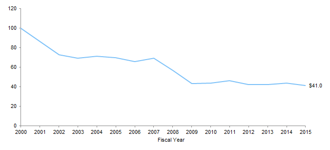
Figure 7. Real Endowment Market Value with a Constant Growth Rule in a Low Return Environment
Fiscal Years 2000–15 • June 30, 2000 = 100
Source: Cambridge Associates Endowment Spending Model.
Notes: This scenario assumes a starting endowment market value of $100 million on June 30, 2000. Spending in year one is equal to 5% of the starting endowment value and subsequent annual spending distributions are increased at the rate of the Consumer Price Index. Portfolio evaluated is 70% US equities (Russell 3000® Index), 30% US bonds (Barclays Government/Credit Index).
Conversely, in a high return environment, a strict constant growth rule can be perceived as significantly under-spending. Figure 8 analyzes effective spending rates[5]The effective spending rate is calculated as total spending for the fiscal year divided by the endowment’s beginning year market value. for the same 70/30 simple portfolio over the trailing 15-year period ending June 30, 2000, which produced a real return of 11.2%. This scenario again assumes a 5% spending rate in year one with all future distributions increasing at the inflation rate. By year 15, the effective spending rate had declined to just 1.7%. This particular shortcoming is pronounced when compared to a market value–based rule that maintained a 5% target spending rate over the same period.
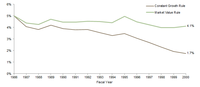
Figure 8. Effective Spending Rates in a High Return Environment
Fiscal Years 1986–2000
Source: Cambridge Associates Endowment Spending Model.
Notes: These scenarios assumes a starting endowment market value of $100 million on June 30, 1985. For the constant growth rule type, spending in year one is equal to 5% of the starting endowment value and subsequent annual spending distributions are increased at the rate of the Consumer Price Index. The market value rule applies a spending rate of 5% to a trailing 12-quarter average market value. The effective spending rate is the amount of spending for the fiscal year divided by the beginning year market value of the portfolio. Portfolio evaluated is 70% US equities (Russell 3000® Index), 30% US bonds (Barclays Government/Credit Index).
In practice, institutions mitigate these shortcomings by imposing a spending cap and floor based on a percentage of the endowment’s market value, or a moving average of market values (Figure 6). Spending collars essentially transform the constant growth rule to a market value–based rule in times of significant endowment growth or contraction to avoid a complete disconnect between spending and the endowment market value. When the constant growth rate falls behind endowment growth by a certain amount, the floor is triggered and the spending distribution is raised to a new level determined by the floor. The cap works in the opposite manner by resetting spending to a lower level than was calculated from the growth measure. Spending caps are typically triggered during periods where the endowment’s market value has significantly declined.
Hybrid Policies
A hybrid spending policy blends the more predictable spending element of a constant growth policy with the asset preservation principle of a market value–based policy and allows an institution to set the mix that best meets its needs. The rule is expressed as a weighted average of a constant growth rule and a percentage of market value (or average market value over a period of time) rule.
An important decision with the hybrid rule is to determine the weighting of the market value and constant growth components. The larger the weighting to the market value component, the more impact a change in the endowment’s market value will have on the annual spending distribution. Most institutions apply the larger weighting to the constant growth component, emphasizing more predictable spending. Half of respondents that use this rule type assign a 70% weighting to the constant growth portion and a 30% weighting to the market value–based portion (Figure 9). Among institutions in this study, the constant growth component is most frequently linked to an inflation index. For the market value component, nearly half of participants used a 5% spending rate. Inputs to the calculation of both the constant growth and market value–based components are shown in Figure 9.
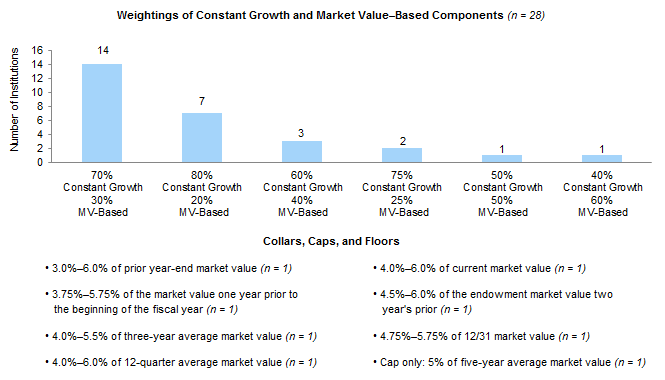
Figure 9. Characteristics of Hybrid Spending Policies
2015
Source: Spending policy data as reported to Cambridge Associates LLC.
Notes: Hybrid policies essentially have the effect of spending a prespecified percentage of an exponentially weighted average market value (MV). The rule is expressed as a weighted average of a constant growth policy and a percentage of market value policy. Of the 28 institutions that use a hybrid spending policy, 20 do not use a collar, cap, or floor to contain year-to-year spending.
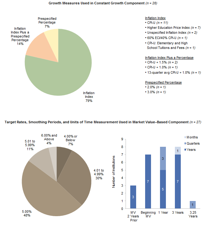
Figure 9 (continued). Characteristics of Hybrid Spending Policies
2015
Source: Spending policy data as reported to Cambridge Associates LLC.
Notes: A hybrid rule is expressed as a weighted average of a constant growth policy and a percentage of market value policy. One institution that uses a hybrid policy did not provide details for the mechanics of the market value–based component of its rule.
Support of Operations
Since few nonprofit institutions generate enough revenue from their core operations to break even on their annual operating budgets, many rely on their LTIP to provide additional financial support. The level of LTIP support varies considerably among the institutions in this study. Spending distributions supported 1% or less of the operating budget for some institutions, while for others it is the single largest source of revenue.
Public universities, which receive financial support from state appropriations, generally rely less on the LTIP to fund the operating budget compared to private colleges/universities and other nonprofits. For the 27 public universities that provided data, median support from the LTIP as a percentage of operating expenses was 2.6% in 2015. Median support for private colleges and university institutions was 12.4% (Figure 10). Among cultural and environmental institutions and independent schools, reliance on the LTIP is higher, as median support of the operating budget was 25.7% and 24.1%, respectively.

Figure 10. LTIP Support of Operations by Institution Type
2015 • Percent (%)
Source: Spending policy data as reported to Cambridge Associates LLC.
Notes: LTIP support of operations is the proportion of the operating budget that is funded from LTIP payout. For the three health care institutions and nine other nonprofits that provided data, LTIP support of operations averaged 36.8% and 42.4%, respectively.
The more predictable stream of spending dollars presumably makes the constant growth and hybrid rules appealing to institutions with higher reliance on the LTIP. Median LTIP support was 26.3% for institutions using a constant growth policy, the highest among the three main rule types (Figure 11). Institutions using hybrid policies, which also contain a constant growth component, had the second highest median LTIP support (17.5%). For institutions using a market value–based policy, median LTIP support was just 8.4%.
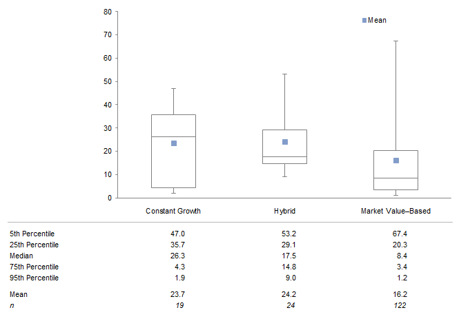
Figure 11. LTIP Support of Operations by Spending Rule Type
2015 • Percent (%)
Source: Spending policy data as reported to Cambridge Associates LLC.
Note: LTIP support of operations is the proportion of the operating budget that is funded from LTIP payout.
Considerations When Setting a Spending Policy
A spending policy is a balancing act between goals for endowment spending and market value growth. Spending policy choices often present tradeoffs, particularly in low returning investment environments when consistent spending erodes market value, or commitment to market value preservation requires reductions in annual spending. An effective spending policy reflects the endowment’s key objectives and its role in supporting the institution. For the purposes of this analysis we consider two key priorities:
- Endowment provides a consistent source of operating revenue for present and future generations.
- Endowment is intended to preserve or grow purchasing power, defined as asset growth that keeps pace with or exceeds inflation.
While these objectives are not mutually exclusive, their attainment may require periodic tradeoffs. Most institutions choose spending policies that strike a balance between these two goals.
Spending Rule Type. Spending policy decisions are often influenced by endowment dependence (the proportion of the budget that is funded from the endowment distribution) and the institutional and donor sensitivity to protecting the endowment’s market value, particularly during steep market declines. Figure 12 compares the annual distributions from a single endowment fund over the last 30 years under three separate spending rule scenarios. The target spending rate, or midpoint of the spending cap and floor in the case of the constant growth rule, is 5% across each of the rule types. The market values from the three scenarios trend in the same direction. The constant growth and hybrid scenarios end the 30-year period with nearly the same market value, while the market value–based scenario is slightly lower.

Figure 12. Endowment Spending and Market Value Under Various Spending Rules
Fiscal Years 1986–2015
Source: Cambridge Associates Endowment Spending Model.
Notes: All scenarios assume a starting endowment market value of $100 million on June 30, 1985. The market value rule applies a spending rate of 5% to a trailing 12-quarter average market value. The constant growth rule distributes 5% of the endowment market value in year one and increases annual spending at the rate of the CPI, with spending levels reset to a cap (5.5%) and floor (4.5%) of a 12-quarter trailing endowment market value where applicable. The hybrid rule distributes 5% of the endowment market value in year one and is a blended rule that uses the Consumer Price Index for the constant growth portion (70% weighting) and 5% of a trailing 12-quarter traililng average market value for the market value portion (30% weighting). Portfolio evaluated is 70% US equities (Russell 3000® Index), 30% US bonds (Barclays Government/Credit Index).
The market value–based rule maintains the strongest link between the portfolio’s market value and its annual spending distributions. This rule produced the highest annual spending distributions during the high return environment of the first 15 years, but was also the quickest to respond to the turbulent market environment of the second 15 years. Spending distributions from this rule were cut substantially following the 2001 and 2008 market declines, but rebounded in the ensuing recoveries. This rule type could be suitable for institutions that want to grow spending when the portfolio benefits from strong performance and restrict spending increases during periods when the portfolio value declines.
The constant growth and hybrid rules result in smoother annual spending distributions relative to the market value rule because the inflationary growth factor is less volatile than investment performance. This effect is particularly evident during the second half of the 30-year period when the variation in annual spending was more moderate compared to the dramatic changes produced by the market value–based rule. The constant growth and hybrid rule types could be preferable for institutions that have a high dependence on the endowment for budget support, and for which substantial fluctuations in annual spending distributions are less tolerable.
Spending Rule Levers. Regardless of the rule type selected, a key decision that an institution must make in setting its spending policy is selecting the appropriate target spending rate, or spending cap and floor (collar) in the case of a constant growth rule. The target spending rate impacts the amount distributed from the portfolio in the present, and has implications for future portfolio growth and future spending. While a lower spending rate results in lower distributions in the present, this fosters a higher portfolio growth rate and eventually leads to higher spending distributions in the long run.
If an institution has a limited reliance on the endowment in the present, or plans for the endowment to play a bigger role in supporting operations in the future, it may want to target a lower spending rate today to enable it to make higher distributions in the future. On the other hand, institutions that already have a high dependence on endowment may seek more of a balance in funding for current and future generations, and therefore pursue a spending rate that more resembles its portfolio’s long-term real return expectation.
As discussed earlier in this report, there are other levers that institutions must define when setting its spending policy. The smoothing period that is applied to the target spending rate or spending collar is the basis for the average endowment value used in the spending distribution calculation. The longer the smoothing period, the less impact that that any one period has in the spending calculation, reducing the year-to-year spending volatility. If using a constant growth rule, an institution must define the growth rate that determines the annual increases in spending. More predictable spending is derived from constant growth rules with a fixed annual increase in spending rather than those linked to inflation, which is not a constant number and is only known in hindsight. And institutions using a hybrid rule assign weightings to the market value and constant growth components, placing the higher weighting on the rule type whose tendencies are prioritized most.
Intergenerational Equity
The goal of intergenerational equity is most often described as maintaining the real purchasing power of the endowment across generations of beneficiaries to ensure all receive equitable support. Institutions that pursue this definition of intergenerational equity would craft a spending policy that aligns with their investment return and inflation expectations. While setting a current spending policy that matches future inflation-adjusted returns is a difficult enough task over the long term, it is virtually impossible over shorter-term periods since returns don’t move in a linear trend. Implementing a policy with the flexibility for year-to-year spending rate calibrations to match investment performance would be impractical for several reasons. Perhaps most significantly, the unpredictable spending that would result would be counterproductive to stakeholders that rely on the endowment to be a consistent source of support.
Figure 13 analyzes spending scenarios for two separate return environments and illustrates the track of real endowment market values for each of the three main spending rule types. With the target spending rate (or midpoint of the spending cap and floor for the constant growth rule) set at 5%, none of the spending rules produced anything that resembled intergenerational equity from a market value perspective in either period. In the high return environment from 1985 to 2000, each rule type ended the period with a real portfolio value that was more than double its starting value. In the low return environment of 2000 to 2015, all three rules types had an ending market value that was at least 25% below its initial value.

Figure 13. Real Endowment Market Values in a High Return vs Low Return Environment
Real Market Value • US Dollar (millions)
Source: Cambridge Associates Endowment Spending Model.
Notes: All scenarios assume a starting endowment market value of $100 million at the beginning of the period. The market value rule applies a spending rate of 5% to a trailing 12-quarter average market value. The constant growth rule distributes 5% of the endowment market value in year one and increases annual spending at the rate of the Consumer Price Index, with spending levels reset to a cap (5.5%) and floor (4.5%) of a 12-quarter trailing endowment market value where applicable. The hybrid rule distributes 5% of the endowment market value in year one and is a blended rule that uses the CPI for the constant growth portion (70% weighting) and 5% of a trailing 12-quarter traililng average market value for the market value portion (30% weighting). Portfolio evaluated is 70% US equities (Russell 3000® Index), 30% US bonds (Barclays Government/Credit Index).
Another way of defining intergenerational equity is as a consistent value for the endowment distribution. Do the annual distributions provide the same benefit to one generation as the next? This definition of intergenerational equity focuses on spending that keeps pace with inflation.
Figure 14 shows the annual spending distributions modeled for the separate 15-year periods. Real spending distributions doubled over the course of the high return environment, when the real investment return (11.2%) was well above the target spending rate (5%). Conversely, spending distributions trended downward from 2000 to 2015 as the real investment return (3.2%) lagged the target spending rate. A strict constant growth rule that does not use a spending cap and floor would maintain steady real spending regardless of the overall investment environment. But as illustrated earlier in Figures 7 and 8, such a policy can jeopardize the purchasing power of the endowment in low return environments and shortchange future generations that could benefit when the endowment earns exceptional returns.
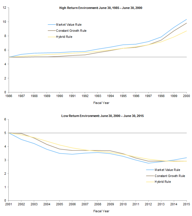
Figure 14. Real Annual Spending Distributions in a High Return vs Low Return Environment
Real Annual Spending • US Dollar (millions)
Source: Cambridge Associates Endowment Spending Model.
Notes: All scenarios assume a starting endowment market value of $100 million at the beginning of the period. The market value rule applies a spending rate of 5% to a trailing 12-quarter average market value. The constant growth rule distributes 5% of the endowment market value in year one and increases annual spending at the rate of the Consumer Price Index, with spending levels reset to a cap (5.5%) and floor (4.5%) of a 12-quarter trailing endowment market value where applicable. The hybrid rule distributes 5% of the endowment market value in year one and is a blended rule that uses the CPI for the constant growth portion (70% weighting) and 5% of a trailing 12-quarter traililng average market value for the market value portion (30% weighting). Portfolio evaluated is 70% US equities (Russell 3000® Index), 30% US bonds (Barclays Government/Credit Index).
In practice for most institutions in this study, the LTIP includes a collection of individual endowment funds. These funds are established at separate points in time, making it unfeasible to pursue the same level of intergenerational equity for each individual fund. The track of an individual endowment fund and its distributions will be highly dependent on the point in the market cycle at which it is created. While the approach to setting a spending policy focuses on the overall LTIP, some individual endowment funds come with donor stipulations that reduce or even halt spending when the market value falls below the original gift value. Such a policy can help an endowment rebuild its purchasing power sooner, but with the tradeoff of disrupting the consistent spending that is also associated with intergenerational equity.
Looking Back and Looking Ahead
At what rate have institutions actually spent from their LTIP? The effective spending rate can help answer this question. The effective spending rate is calculated as the total annual spending distribution as a percentage of the beginning market value of the LTIP. For the 114 institutions that provided effective spending rates over the trailing ten-year period, rates averaged 4.5% in 2015 (Figure 15).
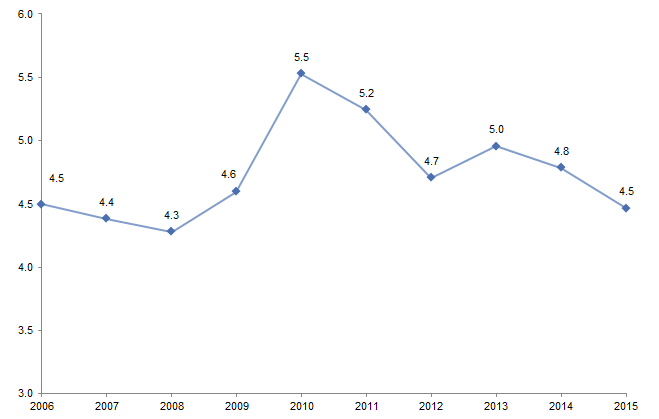
Figure 15. Mean Annual Effective Spending Rate
2006–15 • Percent (%)
Source: Spending data as reported to Cambridge Associates LLC.
Note: Data represent the average of 114 institutions that provided effective spending rates for each year from 2006 to 2015.
While the effective spending rate calculation is based on the most recent year’s beginning LTIP market value, most institutions use an average market value that spans multiple years when determining the annual spending distribution. When the most recent market value is higher than the average market value from the smoothing period, the effective spending rate will be lower than the target rate in the spending policy, and vice versa. Figure 15 shows this inverse relationship between the directional trend of effective spending rates and LTIP growth rates. Effective spending rates spiked upward in 2009–10 as steep portfolio declines resulting from the global financial crisis began factoring into spending policy calculations. Since 2010, average effective spending rates have declined in four of the five years as market values have trended higher.
Six institutions indicated that they have made spending policy changes that will be implemented in 2016 or beyond, each with the intention of lowering the spending rate or collar. Another nine institutions are in the process of considering policy changes that have yet to be approved, five of which are targeting a lower spending rate (Figure 16).
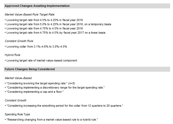
Figure 16. Future Changes to Spending Policies
2016 and Beyond
Source: Spending policy data as reported to Cambridge Associates LLC.
The policies employed by the institutions in this study serve as successful guideposts for a long-term spending policy approach. Since many endowments are considered permanent funds, an institution should set a spending policy for its LTIP that gives it the best chance of sustaining its role in perpetuity. Changes to long-term investment expectations warrant conducting a close evaluation of the spending policy to determine whether the portfolio can still fulfill that defined role. If the perception of a future lower return investment environment persists, more institutions will likely consider policy changes that target lower rates of spending going forward.
William Prout, Investment Director
Tracy Filosa, Managing Director
Footnotes