Annual distributions from the endowment are a source of supplemental operating revenue for most endowed institutions. An institution’s endowment spending policy provides a basis for the calculation of the annual distribution, serving as a bridge that links the long-term investment portfolio (LTIP) and the enterprise. Spending policies are designed to reflect the needs of current and future generations of stakeholders, balancing the goals of providing appropriate levels of support to current operations and preserving, or even growing, endowment purchasing power.[1]Purchasing power is defined as the real market value of the endowment. An endowment that is maintaining purchasing power is keeping pace with inflation (after spending and investment returns). An … Continue reading
The data and analysis in this report cover a variety of spending topics including spending rule types, the endowment’s support of operations, and effective spending rates. This year’s report draws on a supplemental study Cambridge Associates conducted in April 2018 to dive deeper into some technical factors of spending policy, specifically focusing on spending from new endowment gifts.
Annual Review
Cambridge Associates collected spending policy data on 250 of our endowment clients in 2017, including 155 colleges and universities; 37 cultural and environmental institutions; 23 independent schools; 11 health care organizations; and 24 other nonprofit institutions. Foundations were excluded from the survey group as their spending is influenced by certain government-mandated spending requirements. A list of participants can be found at the end of the report. Figure 1 shows the distribution of these institutions across various asset size bands.
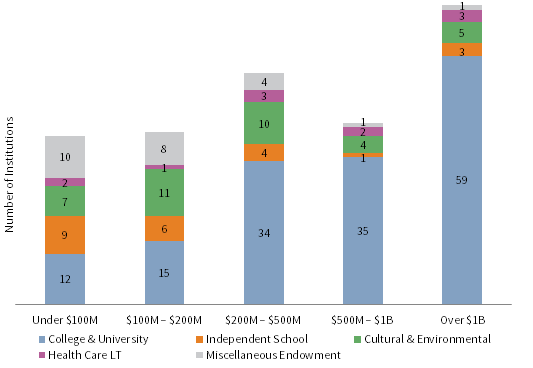
FIGURE 1. PROFILE OF PARTICIPATING INSTITUTIONS
2017
Source: Spending policy data as reported to Cambridge Associates LLC.
Institutions in this study use three primary spending rule types. Market value–based rules link the spending amount directly to the endowment’s market value. Constant growth rules increase spending each year by a defined growth factor. Hybrid policies combine the elements of both market value–based and constant growth rule types.
Figure 2 shows the prevalence of the spending rule types across participating institutions. The most frequently used rule type is a market value–based policy, cited by 76% of institutions. Market value–based rules are most common among the smallest portfolios, with nearly 90% of institutions with assets under $200 million using this approach. In comparison, 56% of institutions with assets over $1 billion use a market value–based rule. Hybrid and constant growth rules were cited by 12% and 9% of all participants, respectively. Both rule types were more likely to be used by larger portfolios than smaller portfolios. Among the institutions with assets over $1 billion, 24% used a hybrid policy and 15% used a constant growth policy.
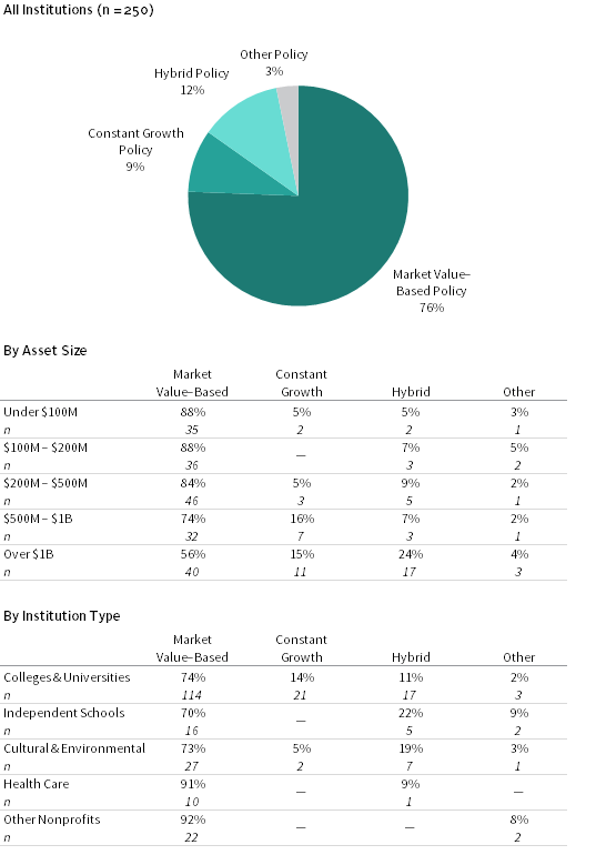
FIGURE 2. SPENDING POLICY TYPES
2017
Source: Spending policy data as reported to Cambridge Associates LLC.
Notes: Market value–based spending policies base spending on a pre-specified percentage of a moving average of market values. Constant growth policies increase prior year’s spending by a measure of inflation and/or pre-specified percentage. Hybrid policies are those that incorporate a weighted average of a constant growth rule and a percentage of market value rule. Other policies are those that cannot be classified as market value–based, constant growth, or hybrid policies.
Figure 3 shows the distribution of rule types for the 140 institutions that provided spending policy data in 2012 and 2017. The market value–based rule continues to be the most common among institutions in this study, with close to the same number of institutions using this policy in 2017 compared to five years ago. Among the other rule types, three more institutions used a hybrid policy; the same number of institutions used a constant growth policy; and one fewer institution used some other policy.

FIGURE 3. SPENDING POLICY TYPES: 2012 vs 2017
n = 140
Source: Spending policy data as reported to Cambridge Associates LLC.
Note: Chart represents the 140 institutions that provided a spending policy in both 2012 and 2017.
Market Value–Based Rules
A market value–based rule dictates spending a percentage of a moving average of endowment market values. By linking the spending distribution amount directly to the endowment’s market value, this rule type usually produces the most dramatic changes in spending when investment conditions shift. Therefore, purchasing power preservation is prioritized during periods when the endowment’s market value declines.
The primary levers of this approach are the target spending rate and the date or smoothing period used to measure the market value. Some institutions also use a cap and floor to contain changes in annual spending during volatile market periods.
Target Spending Rate. The target spending rate helps determine the proportion of the endowment that is distributed on an annual basis. Institutions incorporate long-term investment return expectations and inflation into the selection of the appropriate target spending rate. To preserve the purchasing power of an endowment,[2]In this instance, we use the term “endowment” to refer to a single fund with no future inflows. The LTIP, which is a collection of multiple endowments and other long-term funds, can use inflows … Continue reading the spending rate would align with long-term real investment return expectations. The purchasing power of an endowment will increase when the spending rate is lower than the long-term real return, and vice versa.
In 2017, the majority (88%) of participating institutions that cited a market value–based rule used a pre-specified target rate while the remaining institutions allowed some discretion by setting a pre-specified percentage range within which the target spending rate may fall. For the purposes of comparing target spending rates, we assume the midpoint for institutions that specified a discretionary range. Of institutions with a market value–based policy, 46% used a target spending rate of 5%, while 45% of respondents used a target rate below 5%. Only 9% of institutions applied a rate that exceeded 5% (Figure 4).

FIGURE 4. TARGET RATES USED IN MARKET VALUE–BASED SPENDING POLICIES
2017
Source: Spending policy data as reported to Cambridge Associates LLC.
Notes: Market value–based spending policies base spending on a pre-specified percentage of a moving average of market values. Chart reflects data for the 186 institutions that provided detailed data on their target spending rate. If a range was provided, the target spending rate was calculated using the midpoint of the range.
In fiscal year 2017, 86% used the same target spending rate as reported in the previous year (Figure 5). This is consistent with the trend we have observed over the last five years, where the vast majority of institutions make no change in any given year. Approximately 9% of institutions decreased their target spending rate in 2017 while another 5% increased the rate.
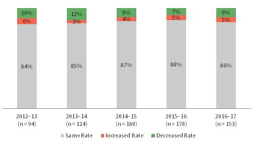
FIGURE 5. INSTITUTIONS CHANGING TARGET RATES IN MARKET VALUE–BASED SPENDING POLICIES
Fiscal Years 2012–17 • Percent (%)
Source: Spending policy data as reported to Cambridge Associates LLC.
Notes: Market value–based spending policies base spending on a pre-specified percentage of a moving average of market values. Chart reflects data for the institutions using a market value–based spending policy that provided the target rate used in their spending calculation. If a range was provided, the target spending rate was calculated using the midpoint of the range.
Smoothing Period. The spending distribution under a market value–based rule is determined by applying the target spending rate to the endowment’s market value. This is usually measured as an average market value over a period of time, known as a smoothing period. By capturing the endowment’s market value over several points in time, the smoothing period helps reduce the year-to-year volatility in spending distributions. Smoothing periods for participants in this report range from one to seven years and the time interval (i.e., monthly, quarterly, or annual market values) can vary (Figure 6). The most common measurement period continues to be 12 quarters (49% of those with a market value–based policy).

FIGURE 6. SMOOTHING PERIODS FOR MARKET VALUE–BASED SPENDING POLICIES: LENGTH OF PERIOD AND UNIT OF TIME MEASUREMENT
2017 • n = 184
Source: Spending policy data as reported to Cambridge Associates LLC.
Notes: Market value–based spending policies base spending on a pre-specified percentage of a moving average of market values. Unit of time measurement indicates whether spending is calculated using monthly, quarterly, or yearly market values. Chart reflects data for the 184 institutions using a market value–based spending policy that provided the unit of time measurement in their spending calculation.
Cap and Floor. The introduction of a spending floor and/or cap can also serve as a smoothing mechanism for spending dollars by limiting the change in spending during particularly volatile periods. A floor for a market value–based rule prevents spending from falling below a certain level, usually the previous year’s spending dollar amount. Although a floor can relieve budgetary pressures during market downturns for institutions with concerns about spending cuts, limiting the decline in distributions can further erode the endowment’s market value and thus make purchasing power preservation more challenging over the long run. A cap limits spending increases when endowment growth is particularly strong by setting a maximum annual growth rate. When paired together, a cap and floor (known as a collar) can produce smoother distributions by maintaining a level of spending during challenging economic environments and saving a greater portion of investment gains from period with exceptional endowment growth.
In practice, only 14 institutions (8%) that use a market value rule employ a cap and/or floor. Nine institutions use a cap and/or floor based on a percentage of a prior year’s spending distribution, and four institutions apply a cap and/or floor to the endowment’s market value on a specific date. Another institution links its cap to the historical gift value of the endowment (Appendix A). For the 22 institutions that outline a discretionary range for the target spending rate, the range serves as a collar in that it allows institutions to raise the rate of spending in down markets and lower the rate of spending when endowment growth rates are high.
Constant Growth Policies
A constant growth spending policy increases the prior year’s spending amount by a measure of inflation and/or a pre-specified percentage. Institutions tend to use this rule type when the endowment is a significant source of operating revenue and volatility in annual spending is less tolerable. More predictable spending is derived from constant growth rules with a fixed annual increase in spending compared to those linked to inflation, which is not a constant number and not known in advance. Of the 23 institutions that use this rule type, 52% use a pre-specified percentage growth rate, 39% use an inflation-index growth rate, and 9% use an inflation-index growth rate plus a pre-specified percentage (Figure 7).
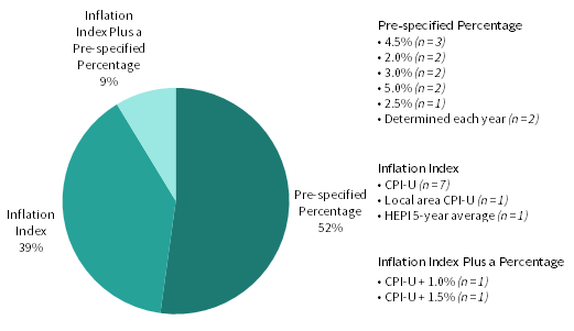
FIGURE 7. GROWTH RATES USED IN CONSTANT GROWTH SPENDING POLICY CALCULATION
2017 • n = 23
Source: Spending policy data as reported to Cambridge Associates LLC.
Note: Constant growth policies increase prior year’s spending by a measure of inflation and/or a pre-specified percentage.
The strict application of a constant growth rule produces predictable spending, but this rule type has some notable shortcomings. Increasing spending during prolonged periods of low or negative investment returns quickly eats away at an already dwindling market value and may permanently impair the endowment. Conversely, in a high return environment a strict constant growth rule can be perceived as significantly under-spending.
In practice, institutions mitigate these shortcomings by imposing a spending cap and floor based on a percentage of the endowment’s market value, or a moving average of market values (Appendix A). Spending collars essentially transform the constant growth rule to a market value–based rule in times of significant endowment growth or contraction to avoid a complete disconnect between spending and the endowment market value. When the constant growth rate falls behind endowment growth by a certain amount, the floor is triggered and the spending distribution is raised to a new level determined by the floor. The cap works in the opposite manner by resetting spending to a lower level than was what calculated from the growth measure. Spending caps are typically triggered during periods where the endowment’s market value has significantly declined.
Hybrid Policies
A hybrid spending policy blends the more predictable spending element of a constant growth policy with the asset preservation principle of a market value–based policy and allows an institution to set the appropriate mix that best meets its needs. The rule is expressed as a weighted average of a constant growth rule and a percentage-of-market-value (or average market value over a period of time) rule.
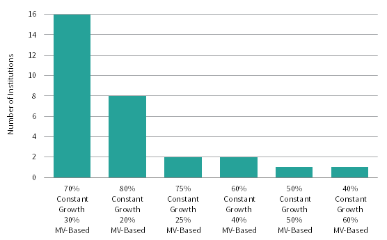
FIGURE 8. HYBRID SPENDING POLICIES: WEIGHTINGS OF CONSTANT GROWTH AND MARKET VALUE–BASED COMPONENTS
2017 • n = 30
Source: Spending policy data as reported to Cambridge Associates LLC.
Notes: Hybrid policies essentially have the effect of spending a pre-specified percentage of an exponentially weighted average market value (MV). The rule is expressed as a weighted average of a constant growth policy and a percentage of market value policy. Of the 30 institutions that use a hybrid spending policy, 22 do not use a collar, cap, or floor to contain year-to-year spending. The eight types of a collar used can be found in the appendix.
An important decision with the hybrid rule is to determine the weighting of the market value and constant growth components. The larger the weighting to the market value component, the more impact that a change in the endowment’s market value will have on the annual spending distribution. Most institutions apply the larger weighting to the constant growth component, emphasizing more predictable spending. Just over half of respondents (16 of 30) that use this rule type assign a 70% weighting to the constant growth portion and a 30% weighting to the market value–based portion (Figure 8). Among institutions in this study, the constant growth component is most frequently linked to an inflation index. For the market value component, the most common target spending rate is 5% (41%). Inputs to the calculation of both the constant growth and market value–based components are shown in Figure 9.
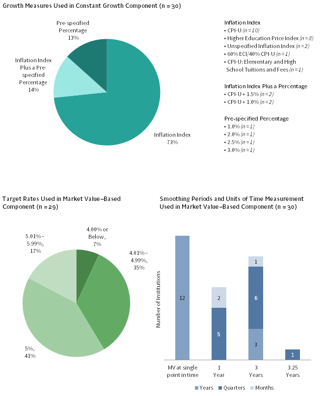
FIGURE 9. HYBRID SPENDING POLICIES: GROWTH & MARKET VALUE–BASED CHARACTERISTICS
2017
Source: Spending policy data as reported to Cambridge Associates LLC.
Notes: A hybrid rule is expressed as a weighted average of a constant growth policy and a percentage of market value policy. One institution that uses a hybrid policy did not provide details for the mechanics of the market value–based component of its rule. Of the 12 institutions using a single market value, one uses the current fiscal year-end market value, four use the beginning fiscal year market value, four use the prior calendar year-end market value, and three use the market value two years prior.
Support of Operations
Since few nonprofit institutions generate enough revenues from their core operations to break even on their annual operating budgets, many rely on their LTIP to provide additional financial support. The level of LTIP support varies considerably among the institutions in this study. Spending distributions supported 1% or less of the operating budget for some institutions, but for others, they serve as the single largest source of revenue.
Public universities, which receive financial support from state appropriations, generally rely less on the LTIP to fund the operating budget compared to private colleges and universities and other nonprofits. For the 22 public universities that provided data, median support from the LTIP as a percentage of operating expenses was 2.8% in 2017. Median support for private colleges and university institutions was 11.6% (Figure 10). Among independent schools and cultural and environmental institutions, reliance on the LTIP is higher, as median support of the operating budget was 18.7% and 19.3%, respectively.

FIGURE 10. LTIP SUPPORT OF OPERATIONS BY INSTITUTION TYPE
2017 • Percent (%)
Source: Spending policy data as reported to Cambridge Associates LLC.
The more predictable stream of spending dollars presumably makes the constant growth and hybrid rules appealing to institutions with higher reliance on the LTIP. Median LTIP support was 26.7% for institutions using a constant growth policy, the highest among the three main rule types (Figure 11). Institutions using hybrid policies, which also contain a constant growth component, had the second highest median LTIP support (22.1%). For institutions using a market value–based policy, median LTIP support was just 8.3%.
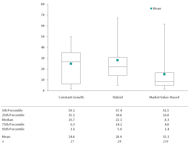
FIGURE 11. LTIP SUPPORT OF OPERATIONS BY SPENDING RULE TYPE
2017 • Percent (%)
Source: Spending policy data as reported to Cambridge Associates LLC.
Notes: LTIP support of operations is the proportion of the operating budget that is funded from LTIP payout. For the three institutions that reported “other” spending policies, LTIP support of operations averaged 40.9%.
Effective Spending Rates
At what rate have institutions actually spent from their LTIP? The effective spending rate can help answer this question. The effective spending rate is calculated as the total annual spending distribution as a percentage of the beginning market value of the LTIP. In 2017 the average effective spending rate was 5.0% for the 111 institutions that provided data for past ten years (Figure 12).

FIGURE 12. MEAN ANNUAL EFFECTIVE SPENDING RATE
2008–17 • Percent (%) • n = 111
Source: Spending data as reported to Cambridge Associates LLC.
Note: Data represent the average of 111 institutions that provided effective spending rates for each year from 2008 to 2017.
Though the effective spending rate calculation is based on the most recent year’s beginning LTIP market value, most institutions use an average market value that spans multiple years when determining the annual spending distribution. When the most recent market value is higher than the average market value from the smoothing period, the effective spending rate will be lower than the target rate in the spending policy, and vice versa. Figure 12 shows this inverse relationship between the directional trend of effective spending rates and LTIP growth rates. Effective spending rates spiked upward in 2009–10 as steep portfolio declines resulting from the global financial crisis began factoring into spending policy calculations. While average effective spending rates have declined in most years since 2010, the mean ticked up by 10 basis points (bps) in 2016 and by 40 bps in 2017.
Policies on New Gifts
No matter what type of spending rule is used, endowments face the common issue of how to incorporate new gifts into their spending calculation. There are two primary decisions to make about spending from new endowments:
- Whether to institute a deferral period during which a new gift is excluded from the endowment’s spending policy, and
- Whether to make a full or partial distribution from a new gift once spending from the new gift occurs.
There are justifiable reasons that different approaches can be taken on both of these choices. On the one hand, donors often wish to see their dollars put to work as soon as possible and the program supported by a new gift could be limited or constrained until the gift provides its full spending distribution. On the other hand, limiting or deferring spending from a new gift for an initial period will increase the odds that it maintains its purchasing power and will result in more spending dollars available for distribution over the long term.
In April 2018, Cambridge Associates administered a survey that asked institutions about some technical components of the spending distribution calculation, including new gift spending policies.[3]A total of 96 nonprofit institutions responded to the survey, the majority of which were educational endowments (68% colleges & universities and 15% independent schools). In the sections that follow, we review the common approaches that institutions take with new gifts and their spending policy. Also included is an analysis on the impact of these various approaches based on a simulation of spending outcomes during past market environments.
Deferral Periods
Over three-quarters of survey respondents reported that they do not have a deferral period for incorporating new gifts into the spending policy calculation (Figure 13). Without a deferral period, a new gift will be included in the equation when the next spending amount is calculated for the endowment and a distribution will be made from the gift. The benefit of a deferral period is that it can give a new gift additional time to season and potentially grow its purchasing power before distributions begin. Among the institutions that defer spending from new gifts, the most common deferral policy is based on a certain period of time. For those that use a time-based deferral policy, asset growth will only occur if the endowment earns a positive investment return during the deferral period. Only two institutions specified that a minimum asset growth threshold must be met before the initial spending distribution can be taken from a new gift. With asset thresholds there is uncertainty around when the initial spending will occur, as the timing is dependent on future investment performance.
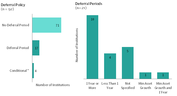
FIGURE 13. DEFERRAL POLICIES FOR NEW ENDOWMENT GIFTS
Source: Spending data as reported to Cambridge Associates LLC.
Note: A deferral period refers to an instance where a new gift is not included in the first spending policy calculation that occurs after the gift is received.
* There is a deferral policy, only if a new gift is received after a cut-off date.
Initial Distribution Level
The question of whether to spend a full or partial amount at the first spending distribution is more complex. Spending from new gifts for almost all institutions is based on some percentage calculation, but this can be a percent of full market value, a percent of the prorated average market value over a smoothing period, or a percent of the original gift amount. A market value–based spending rule offers a relatively simple choice between spending the full policy amount or a partial amount for a new gift. Respondents that use a market value–based rule type were nearly evenly split between these two choices (Figure 14).
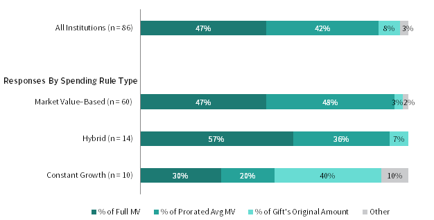
FIGURE 14. INITIAL DISTRIBUTION LEVEL FROM A NEW GIFT
2017
Source: Spending data as reported to Cambridge Associates LLC.
Note: Two institutions that use an other spending rule type are included in the all institutions breakout, but are not listed in the section by spending rule type.
Spending a percentage of a new gift’s full market value is most common for institutions that unitize their endowment funds and calculate a uniform spending-per-unit amount. In this instance, all gifts, regardless of how long they have been in existence, would spend an equal amount in proportion to their respective asset sizes at the distribution date. A gift that has existed for just two quarters would realize the same spending potential as other endowment funds that have existed for the entire smoothing period.
Institutions that base spending from new gifts upon a percentage of the gift’s prorated average market value use a more strict application of the smoothing period. For example, if the smoothing period is 12 quarters and a new gift has existed for only one quarter, the spending amount from the new gift would be the spending rate multiplied by one-twelfth of the gift’s average historical market value. Under this scenario, a new gift only reaches its full spending potential once it has existed for the entire smoothing period.
The hybrid and constant growth rule types incorporate an inflationary component where at least a portion of the annual spending distribution is based on some predetermined growth rate. While a smoothing period is often still a component of the policy, respondents using these rule types were less likely to base the initial spending amount on the prorated average market value of the new gift. Most of these respondents set a rate at which to start spending, either based on the market value at the time of the initial distribution or the original gift value.
Impact of Policy Choices
The decisions that institutions make about initial spending from new gifts will have an impact on the future asset growth and spending from the gift. To study this further, we modeled scenarios that assess the impact of these decisions. Figure 15 considers the decision of whether to spend the full amount right away from a new gift or to institute a deferral period.
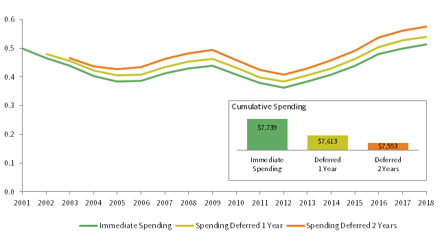
FIGURE 15. NEW GIFT SPENDING METHODOLOGY: IMMEDIATE SPENDING VS DEFERRAL POLICY
2001–18 • Nominal Annual Spending in USD millions
Source: Cambridge Associates LLC Spending Model.
Notes: Analysis begins with a $10 million endowed gift invested on June 30, 2000. Growth of the gift is based on a 70/30 portfolio, rebalanced annually, composed of the MSCI World Index and BBG Barclays Government/Credit Bond Index. Spending is based on 5% of a 12-quarter historical market value from 2004 to 2018 for all scenarios. For the years 2001 through 2003, the following policies are used: Immediate Spending – spend 5% of the entire historical average quarterly market value that is available; Deferred 1 Year – no spending in 2001, then spend 5% of the entire historical average quarterly market value that is available; Deferred 2 Years – no spending in 2001 or 2002, then spend 5% of the entire historical average quarterly market value that is available.
In the immediate spending scenario, the spending policy applied the 5% spending rate to the full market value in the first fiscal year. Since this policy began distributing a full spending amount right away, asset growth for the gift lagged that of other scenarios where spending was deferred. The lower asset base results in lower annual distributions compared to the deferred policies. Although this policy produced the highest cumulative amount of spending for the 18-year period, that cumulative amount will eventually fall behind that of the other scenarios as it continues to produce the lowest annual distributions in the future.
Two scenarios modeled used a deferral period. One scenario skipped the spending distribution in the first fiscal year and the other skipped spending in the first two fiscal years. By the third fiscal year, all three scenarios in the illustration were using the same spending rate and smoothing period. Since money was not taken out on the first spending date, both of the deferred policies resulted in higher asset values and spending distributions in subsequent years compared to the immediate spending scenario. A similar effect is evident when comparing the two deferred policies, as the policy with the longer deferral period resulted in a larger asset base and higher annual spending. For more detail on this, see Appendix B.
A spending policy with a deferral period will provide greater purchasing power and yield more spending dollars over the very long term. Extending the deferral period favors the long-term impact at the expense of the more immediate term (Figure 16). In deciding whether to institute a deferral period for new gifts, institutions need to consider the trade-offs between making an immediate impact versus having a greater impact over the long term.

FIGURE 16. DEFERRAL PERIODS PRIORITIZE LONG-TERM IMPACT OVER IMMEDIATE IMPACT
Source: Cambridge Associates LLC.
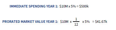
Figure 17 considers the decision of whether to spend a full or partial amount from a new gift at the time of the first spending distribution. The immediate spending scenario is the same that was used in the first analysis. For the first three annual spending distributions, this scenario applied the 5% spending rate to the full historical average market value even though the gift hadn’t existed for the entire 12-quarter smoothing period. In contrast under the prorated market value scenario, the 5% spending rate is multiplied by n/12 of the gift’s average quarterly market value where n equals the number of historical quarter-end dates that the gift has existed. For example, in year one where the gift had just one quarterly market value in its history, the spending distributions were calculated as follows:
The prorated market value scenario gradually increases spending in the early years after the gift is established. By year four (2004), a full 12-quarter market value history was available and both policies transformed to the normal spending rule. Since the prorated market value scenario produced the least amount of spending during the first three years, it resulted in a larger asset base and higher annual spending distributions relative to the immediate spending scenario in all subsequent years. While the prorated policy produced a lower cumulative amount of spending for the full period, that cumulative amount will eventually surpass the immediate spending scenario as it continues to produce the highest annual spending distributions into the future. For more detail, see Appendix B.
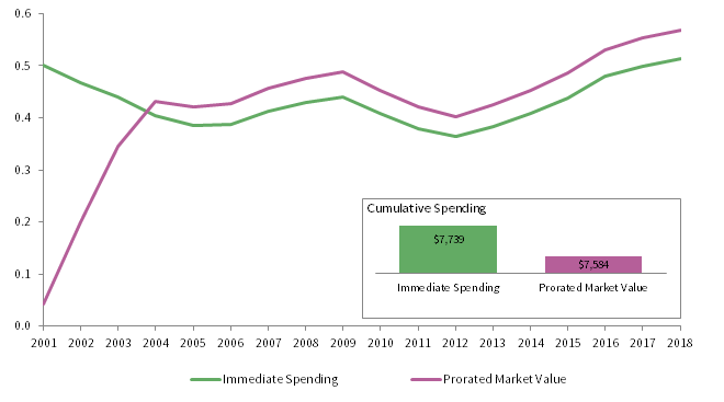
FIGURE 17. NEW GIFT SPENDING METHODOLOGY: IMMEDIATE SPENDING VS GRADUAL APPROACH
2001–18 • Nominal Annual Spending in USD millions
Source: Cambridge Associates LLC Spending Model.
Notes: Analysis begins with a $10 million endowed gift invested on June 30, 2000. Growth of the gift is based on a 70/30 portfolio, rebalanced annually, composed of the MSCI World Index and BBG Barclays Government/Credit Bond Index. Spending is based on 5% of a 12-quarter historical market value from 2004 to 2018 for both scenarios. For the years 2001 through 2003, the following policies are used: Prorated Market Value – spend 5% of n/12 of the gift’s average quarterly market value where n equals the number of quarters that the gift has existed; Immediate Spending – spend 5% of the entire historical average quarterly market value that is available.
A Note on Underwater Endowments:
Our historical analysis of spending outcomes in this paper begins near the stock market peak of the Dot-com bubble in 2000. In each of the scenarios we analyzed, the new gift fell below its original dollar value (“underwater”) almost immediately and the asset value remained underwater for most of the fiscal years in the model period. A survey we administered to colleges and universities in 2016 revealed that most respondents (62%) continue using the normal spending rule when an endowment falls underwater. However, a significant proportion (26%) immediately modify their spending in some way when an endowment falls underwater and another 11% of respondents modify their spending once an endowment falls a certain percentage amount below the original gift value.
The scenarios we modeled did not cease or limit spending once the gift fell below its original dollar amount. However, institutions sensitive to this issue could incorporate restrictions on spending from underwater funds as a part of their spending policy. Underwater policies help to protect the purchasing power of endowment funds in poor return environments, but modifying spending can cause disruptions to the programs that underwater endowments support. Please read “Keeping Underwater Endowments Afloat (and the Programs They Support)” for a full discussion on this topic.
Figure 18 compares the spending scenarios across a set of priorities that institutions should consider when designing a new gift spending policy. There is a clear contrast between the immediate spending and deferred spending policies where the key decision is choosing between making an immediate impact versus a greater impact in the long run. If partial spending in the early years is an acceptable outcome, the prorated market value policy can balance a donor’s wishes that the gift be put to use right away, while also setting it up to have a greater impact over the long term. However, one downside to this policy is that it could cause extra administrative burden in the tracking of separate endowment gifts and applying the spending policy on a gift-by-gift level. The same could also be true for policies with a deferral period where new gifts have to be tracked separately for spending purposes for an initial period.
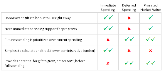
FIGURE 18. COMPARISON OF NEW GIFT SPENDING POLICIES
Source: Cambridge Associates LLC.
Note: One check mark indicates a policy somewhat supports the priority listed, but is not as effective as a policy with two check marks.
Endowment gifts are intended to support an institution and its programs over the long term. Building strong policies around new gift, and ongoing, spending can help ensure that this is the reality. The longer that spending from a gift is deferred, the greater the impact the gift will have in the future. But funds can’t be stashed away forever. Donors want and expect to see an impact from their giving both in the present day and in the future. An institution needs to carefully consider the desires of its donors, the needs of the programs that depend on a new gift, and the long-term sustainability of the gift when designing spending policies for new gifts.
William Prout, Senior Investment Director
Tracy Filosa, Managing Director
Meredith Wyse, Senior Investment Associate
Footnotes