Defined benefit pension plans face ample challenges in the current environment of extremely low interest rates. Most agree that low yields have caused liability-hedging assets (longer-duration fixed income) to become overvalued when evaluated in isolation. However, plans are limited in how to act upon this overvaluation, given the embedded interest rate sensitivity also associated with plan liabilities and funded status risk (also known as “surplus risk).
A plan’s interest rate sensitivity should always be taken into account; however, the current level of interest rates results in a highly asymmetric profile for future fixed income returns and, more importantly, for future changes in a plan’s liability values. These extremely low interest rates result in a reduced risk of further interest rate declines, which means there is a much lower risk of liabilities rising significantly and much lower expected returns for bond holdings. Plan sponsors that ignore this asymmetry may fail to appropriately adjust their asset allocations. As a result, the plan’s future return potential may be degraded, ultimately resulting in the need for significantly higher contributions.
Many market participants advocate de-risking plans, or “glide paths,” whereby exposures and/or risk profiles are adjusted over time based primarily on changes in the funded status. Typically, these glide path blueprints de-risk as funded status increases by re-allocating funds out of the growth assets and into the liability hedge. In normal market environments, such a shift will reduce plan surplus risk but also reduce expected returns. In the current environment of bond overvaluation and historically low yields, this glide path approach results in a significantly larger drop in expected returns that can result in the need for higher contributions into the plan.
We agree that as a plan’s funded status changes, dynamically adjusting asset allocation to maintain targeted levels of surplus risk is appropriate. We also agree that it may be appropriate to adjust the level of surplus risk explicitly at different levels of funded status. However, we believe many glide paths are too mechanical in their approach to risk reduction, with a tendency to rely too much on increasing the fixed income allocation to maintain or dampen surplus risk. By adhering to a risk-reduction process that relies exclusively on increasing the liability hedge and reducing the growth assets, the glide path structure neglects the objective of maximizing return at each targeted level of risk. To achieve superior results, we advocate a more holistic and flexible approach to dynamic asset allocation, making use of multiple risk-reducing levers.
This paper articulates an alternative solution—a flexibly constructed glide path that achieves the competing goals of reducing surplus risk and generating superior returns, while still reducing the risk of a significant decline in funded status. This glide path solution is implemented by reducing directional equity exposure (equity beta) and replacing it with strategies that are driven by alpha and “non-traditional betas” (such as distressed credit, hedge funds, and private investments). As outlined in our 2011 report Pension Risk Management, we believe pension risk-budgeting frameworks that use all levers of risk management, including structuring risk-controlled growth assets, are preferable in most market environments. However, we find the merits of this strategy particularly compelling in the current environment of extremely low bond yields.
The Current Rate Environment
First, some context on the current interest rate environment is useful. We provide a frame of reference on how low current interest rates are compared to prior history and, more importantly, evaluate the implications of these low yields for pension liability values and longer-duration bond returns associated with liability hedges.
U.S. investment-grade interest rates across the yield curve are near generational lows. Interest rates have been driven lower by a pervasive rally in high-quality fixed income securities that has now spanned 31 years. The low level of current yields has resulted in significantly lower discount rates that have driven the present value of defined benefit plan liabilities appreciably higher.
Defined benefit plan discount rates are influenced by two primary forces: The level of general interest rates (proxied by the “risk free” interest rates of U.S. Treasuries) and the relative spread of investment-grade credit securities over Treasuries[1]While we specifically address implications for plans using an investment-grade credit fixed income discount rate for their liabilities, this framework is broadly applicable to any plan that might … Continue reading. For the purpose of explaining our case for a flexible dynamic asset allocation framework, we evaluate a worst-case scenario that could conceivably occur via further drops in investment-grade yields and increases in liability values. Note that, conversely, this would also be considered a best-case return scenario for long-duration bonds held as liability hedges.
U.S. Treasury Rates
Nominal U.S. Treasury yields have plunged to generational lows, a function of Treasuries being purchased as safe haven assets during and after the recent financial crisis, as well as the significant purchases of government bonds by the Federal Reserve. As of December 31, 2012, ten-year nominal Treasuries yielded only 1.76%, nearly 5 percentage points below their 50-year average yield (Figure 1). Similarly extreme, 30-year nominal Treasuries yielded only 2.95%, almost 4 percentage points below their 50-year average.[2]In July 2012, ten- and 30-year Treasury yields hit recent lows of 1.39% and 2.45%, respectively.

Figure 1. U.S. Ten- and 30-Year Treasury Yields
December 31, 1945 – December 31, 2012

With Treasury yields trading at depressed levels (a phenomenon common across government bonds in the developed world), the asymmetry of potential changes in yields is readily evident—Treasury prices possess a finite amount of further appreciation potential versus a far larger amount of downside risk if yields revert higher to more “normal” levels. To help quantify the potential size of further declines in Treasury yields and resulting gains in Treasury prices, and ultimately the related potential upside remaining in plan liabilities, we developed a rate scenario that mimics the behavior of Japanese interest rates, which have plummeted given that country’s ongoing multi-decade deleveraging.
Indeed, Japan has become the modern day example of the depth to which developed world rates can drop—severe deflation, weak economic growth, and the forces of deleveraging continue to beleaguer the country’s economy. The December 31, 2012, yields on ten-, 20-, and 30-year Japanese government bonds (JGBs) were a paltry 0.79%, 1.75%, and 1.98%, respectively (Figure 2).[3]In mid-2003, ten- and 30-year JGBs hit all-time lows of 0.45% and 0.98%, respectively. These lows were short-lived, as yields more than doubled within the next month. The December 31, 2012, yields … Continue reading For the purpose of this analysis, we view these Japanese rates as a reasonable boundary for further downside in nominal Treasury yields, under a hypothetical assumption that the United States follows the same painful Japanese deleveraging path. Assuming this worst-case economic scenario occurred, U.S. ten- and 30-year Treasury yields would both drop an additional 97 basis points (bps).

Figure 2. Japanese Government Bond Ten- and 20-Year Yields
July 3, 1992 – December 31, 2012
Source: Bloomberg L.P.
Such a drop in Treasury yields (assumed instantaneously) would result in only a 14% gain for the Barclays Long Credit Index, a common liability hedge benchmark for many plan sponsors.[4]The Credit Index is influenced by risk-free interest rates, as well as credit spreads in excess of risk-free rates. This particular calculation assumes spreads are constant. If Japan were the appropriate precedent, the 14% return could essentially be considered the best-case scenario for Treasuries, and correspondingly, the worst-case scenario for potential increases in a plan’s liabilities resulting from changes in Treasury yields.[5]Estimated liability change stated here and later in this paper is highly related to an individual plan’s liability duration—plans with lower duration than the index referenced will experience … Continue reading
Conversely, if yields reverted to the higher levels seen in 2007 or 2011, this rate spike would induce a significant decline of 21% to 30% in the index. Importantly, this implies expected declines of a similar magnitude in pension plan liabilities.
U.S. Corporate Credit Spreads
The second factor to examine in this scenario analysis is long-duration credit spreads, given credit-based yields are used as liability discount rates. As of December 31, 2012, the Barclays Long Credit Index yielded near a record low of 4.32% (Figure 3).[6]The Long Credit yield hit its all-time low level of 4.19% on November 13, 2012. However, the decline in absolute credit yields has been driven more by the low levels of Treasuries as opposed to unusually low credit spreads. Indeed, the option-adjusted spread (over similar duration U.S. Treasuries) for Long Credit is 180 bps, about 40 bps higher than the average level going back to 1989. If Treasury rates were held constant and long credit spreads tightened to the 23-year average, the Long Credit Index would gain about 6%, implying a similar increase in pension liabilities resulting from credit spread compression.

Figure 3. Barclays U.S. Long Credit Yield and Option-Adjusted Spread (Over Treasuries)
January 31, 1973 – December 31, 2012
 Sources: Barclays, Barclays POINT, and Bloomberg L.P.
Scale of Potential Liability Increases
If we assume the perfect storm and combine the pension plan’s worst-case scenario for Treasury rates and credit spreads combined—the United States “becomes Japan” as Treasury yields drop 97 bps and credit tightens 40 bps to match average spread levels—the Long Credit Index would increase 21%. Many U.S. plan liabilities have a longer-duration profile similar to the Long Credit Index, and most plans’ discount rates are derived from investment-grade credit yields. Thus, we can reasonably proxy that this worst-case scenario would result in pension liabilities increasing roughly 21%. Although this is a rather unpleasant thought, it is modest and manageable relative to the massive drop in rates and massive increase in liabilities that already occurred in the last decade.
Clearly, plans must maintain caution when choosing to express any kind of asset allocation position based on capital markets expectations, remaining mindful of significant duration sensitivities embedded within pension liabilities. However, it is clear the current environment presents a highly asymmetric profile—plans that elect to increase or maximize liability hedges are doing so at extremely depressed yields and are locking in very low future returns. By earning such low asset returns, larger contributions will ultimately be necessary. Ultimately, plans increasing liability hedges today are doing so at a time when funded status tail risk from potential declines in interest rates is significantly lower, as rates quite simply have less potential for further declines given their already low levels.
Concept of the “Glide Path”
Defined benefit plan sponsors have already faced significant challenges in the current low interest rate environment. As liabilities have increased, the funded status of plans has declined, and plans have been forced to make large contributions. This understandably caused many plans (particularly those that are more risk averse due to broader enterprise-level factors) to focus on better controlling and reducing liability relative risks, which encouraged the design of de-risking “glide paths.”
The core premise for a glide path is that as a plan moves toward being fully funded, the plan can or should assume less risk, while still meeting return targets. De-risking is particularly important given the asymmetric cost/benefit profile of a plan’s funded status. Specifically, if the plan benefits from an outsized increase in its funded status and has a significant surplus, such gains cannot be extracted out of the plan for an extended period of time. Conversely, if the plan experiences outsized declines in its funded status, it necessitates additional and more immediate capital contributions to offset the funded status deterioration. Although recent regulatory relief regarding liability discount rates has temporarily lessened the pain of underfunding, it remains imperative to assess funded status on an economic (“mark-to-market”) basis, as the detriment that results from a funding status shock will ultimately be absorbed by the plan sponsor as the regulatory relief eventually wears off.
A review of the method in which most glide paths have been constructed shows that moving from “Point A” to “Point B” typically involves a shift out of the growth assets into the liability hedge on a straight-line, pro rata basis as the funded status increases. While such de-risking glide path approaches may seem appealing in terms of their simplicity, they often do not define targeted risk or return levels. Additionally, these mechanistic glide paths do not explicitly address the degradation in expected returns that results from shifting allocations out of the growth assets and into the liability hedge. Finally, they often do not appropriately incorporate current market conditions.
We unequivocally agree that as a plan’s funded status changes, it is appropriate to map out targeted risk and return levels. To adjust targeted risk and return levels, there is clearly an associated need to adjust plan exposures. However, we advocate a more holistic approach to de-risking and glide paths.
The Solution—An Alternative Glide Path
A glide path can be constructed to manage and reduce funded status risk via multiple mechanisms as funded status grows. Ultimately, the goal for the glide path should be to maximize expected return at each targeted (and reduced) level of risk. A holistically constructed glide path will:
- Be superior in achieving the dual goals of maximizing returns and reducing targeted funded status volatility; and
- Reduce the risk of a large drawdown in a plan’s funded status.
The more holistic glide path is driven not only by appropriate sizing of the growth assets, but also by defining and controlling the risk within the growth assets. These risk-controlled growth assets emphasize active strategies that rely on manager skill and non-traditional beta over mere directional equity market exposure.
The current environment of extremely low market yields only accentuates the merits of this approach. As already shown, long-duration Treasury yields are very low. Further, including public equities and real assets (we observe that asset classes outside of fixed income) are generally priced at valuations at or above fair value based on long-term metrics. Thus, with muted asset return expectations and a lower risk of a significant decline in discount rates that would cause a significant increase in liability values, we believe higher active risk strategies, such as low-beta hedge fund exposures and select private investment strategies, are capable of offering expected returns that are more attractive from a risk/return perspective.
Glide Path Allocation Comparison
To illustrate our approach, we compare two potential de-risking glide paths. The first uses long-duration bonds[7]For this analysis, the liability hedge is assumed to be long-duration investment-grade corporate bonds. (liability hedge) and publicly traded global equities, with the former growing and the latter shrinking as funded status increases. This asset allocation progression will be referenced as the “Traditional Glide Path” going forward, and is intended to mimic the more mechanical roadmap that many have advocated. The second glide path (Holistic Glide Path) represents an example of a holistic approach that maintains a lower liability hedge than the Traditional Glide Path and incorporates more active strategies such as low-beta hedge fund exposures and select private investments. Our comparison of these two glide paths focuses on their funded status risk and expected returns; we also use historical stress tests to observe each glide path’s performance under real market scenarios. Note that these glide paths target risk levels that may not be appropriate for all plans—in practice, each plan should create a custom glide path based on its unique circumstances and institutional risk tolerance.
Glide Path Risk Comparison
The Holistic Glide Path was intentionally calibrated to match the funded status volatility of the Traditional Glide Path at each point along the funded status continuum. However, the primary difference between the two glide paths is the means through which they seek to de-risk the plan. The Traditional Glide Path de-risks by shifting exposures toward the liability hedge portion as the funded status increases. Conversely, the Holistic Glide Path seeks to de-risk via a combination of increasing the weight of the liability hedge and allocating funds away from public equities to strategies with less equity market risk (“equity beta”) but higher active risk (such as can be found in select low-beta hedge funds). Thus, the Holistic Glide Path holds the immediate advantage of using multiple levers to adjust risk, whereas the Traditional Glide Path has only one lever to adjust risk (Figure 4).
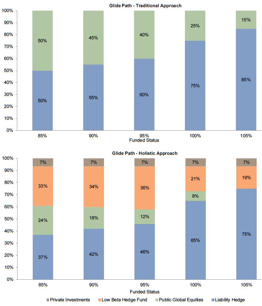
Figure 4. Asset Allocation of Traditional and Holistic Glide Paths at Various Funding Levels
Note: Figures may not total 100 due to rounding.
With multiple levers of risk reduction at each point of the glide path, the Holistic Glide Path generally uses lower amounts of liability hedge compared to the Traditional Glide Path. However, Figure 5 demonstrates that the expected surplus volatility[8]The surplus volatility depicted represents the standard deviation of expected asset returns versus those of the liability. It therefore represents the risk (volatility) of under/overfunding by … Continue reading of the Holistic Glide Path and the Traditional Glide Path is identical at various levels of funded status. Thus, even though the Holistic Glide Path may have up to 14% less invested in the liability hedge, identical risk reduction can be achieved through investment in strategies with lower beta and higher active risk. It is important to point out that there are a number of glide paths that could be constructed with similar volatility; for simplicity, we have chosen to evaluate two very different approaches.

Figure 5. Surplus Volatility
Glide Path Return Comparison
Of course, we acknowledge an alternative de-risking path should only be considered if it is expected to generate higher returns, perform better across a greater diversity of market environments, and/or meaningfully mitigate other forms of risk, such as funded status tail risk. The next step of our analysis uses Cambridge Associates’ long-term equilibrium expected returns for each asset class to determine expected return for the total fund at each point of the competing glide paths.
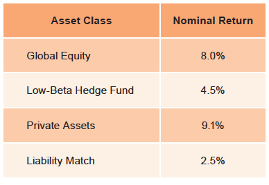
Based on our long-term return assumptions for a “Normal Environment,” the baseline expected return of the Holistic Glide Path is modestly lower than the Traditional Glide Path at each funded status point (Table 1). However, our long-term equilibrium expected returns are based primarily on market beta, and do not include an estimate of manager value add (or “alpha”) beyond any non-traditional beta one might expect from investing in the average manager in these strategies. This is an important omission when discussing strategies such as low-beta long/short equities and arbitrage hedge funds, since a plan’s implementation of these strategies will only be successful if the manager roster generates significant value added.

Table 1. Absolute Nominal Return in Normal Environment
To help incorporate the important component of hedge fund alpha, we have included an additional row in Table 1 labeled as the “Holistic Glide Path + 300 bps Targeted Hedge Fund Alpha,” where we have added what we believe is an appropriate estimate for hedge fund alpha. For reference, Cambridge Associates’ clients with low-beta hedge fund programs generated, on average, approximately 320 bps of average annual alpha for the most recent ten-and-a-half years.[9]Alpha calculation based on the average return of C|A hedge fund advisory programs with beta less than 0.3 (measured relative to MSCI ACWI IMI [net] since program’s inception) for the October 31, … Continue reading If a plan generates this level of hedge fund alpha, the Holistic Glide Path has expected returns higher than the Traditional Glide Path at the same levels of funded-status volatility, as true alpha is an independent component of total return.
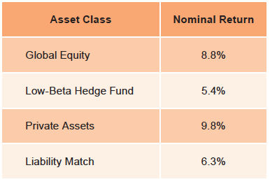
Our long-term return assumptions are based on equilibrium capital market conditions. Unfortunately, the market environment today is not reflective of equilibrium, particularly as it relates to bond yields. For the purpose of this paper, we developed return assumptions for each asset class assuming valuations revert to normal levels over the next ten years (“Current Market Environment”). This addresses the unique valuations embedded in capital markets at present.
In our Current Market Environment analysis, the expected returns for all points on the glide paths are well below 6% (Table 2). These expected returns glaringly highlight the difficulty most plans will face in achieving targeted returns in the current market environment. To hit the targets in this market environment, most plans will either have to take more funded status risk or pursue a different strategic approach, such as the Holistic Glide Path, which is a superior way to generate higher expected returns at a targeted level of funded status volatility.

Table 2. Absolute Nominal Return in Current Market Environment
As shown in our analysis, if a plan can generate the targeted level of hedge fund alpha, the Holistic Glide Path’s expected return is in most cases significantly higher than that of the Traditional Glide Path in the Current Market Environment. Evaluated from a different perspective, expected returns from the Holistic Glide Path (within the Current Market Environment) will equal the Traditional Glide Path if an investor can structure a low-beta hedge fund program that achieves at least 105 bps of alpha.[10]For reference, the average of C|A’s low-beta hedge fund client programs has exceeded this 105 bp alpha hurdle 98% of the time on a rolling three-year basis over the last ten-and-a-half years. Note … Continue reading
A fair criticism of our analysis might be our lack of alpha assumptions for any asset classes other than hedge funds, which may unfairly favor the Holistic Glide Path relative to the Traditional Glide Path. One reason we did not extrapolate an alpha assumption to other asset classes is the fact that many plans implement their liability hedge and equity assets passively (thus, there will be no alpha). While we typically advocate active management in public equity and bonds (as well as tactical positioning), it is clear that alpha assumptions are unique to each plan. For the Traditional Glide Path to achieve expected returns that match those of the Holistic Glide Path (with assumed hedge fund alpha), the Traditional Glide Path would have to garner a substantial amount of alpha on its equity and liability-hedging assets. Using our Current Market Environment assumption at the 90% funded status as a reference, a plan would have to earn 226 bps of alpha on its equity mandates and 100 bps on its bond mandates for the expected return of the Traditional Glide Path to match the expected return of the Holistic Glide Path (with 300 bps of targeted hedge fund alpha).[11]Calculation assumes amount of public equity alpha earned is also earned on private equity and oil gas assets in the holistic allocation. It would be an understatement to call the expectation of such alpha generation for these more efficient asset classes extremely ambitious.
Glide Path Tail-Risk Comparison
Another important distinction between the two glide path approaches is their ability to mitigate significant drawdowns in funded status due to poor market performance. As we have seen over the past decade, large and sudden drops in funded status are painful for plans, as significant increases in contributions are required to offset the large declines in funded status. Risk/return evaluations with forward-looking assumptions are useful exercises, but they fail to take into account the real life impact of drastic funded status drawdowns. The most recent financial crisis provides an excellent stress test, as global equities lost 49% of their value from September 30, 2007, through March 31, 2009.[12]Represents the cumulative return for this period for the MSCI All Country World (Net) Index in US$ terms.
For the purpose of this analysis, we assume a plan starts with a funded status of 90%, and the asset allocation follows the previously described glide paths. Contrary to what many would have expected, the Holistic Glide Path approach better preserved the funded status than the Traditional Glide Path during the most recent crisis (Figure 6). Despite the Holistic Glide Path holding lower liability-hedging assets, it benefited from significantly lower equity beta that resulted from a risk-controlled and diversified growth portfolio—a powerful tail-risk reducer given the extremely poor performance of public equities during this time period.

Figure 6. Funding Level Preservation: Traditional Glide Path Versus Holistic Glide Path
Assumed Initial Funding Level of 90%
As a final component of our analysis, we compare the two approaches in a strongly positive environment for equity markets with moderately rising discount rates (to isolate the low-beta effect of the Holistic Glide Path). For this purpose, we use the three-year period ending December 31, 2007, when global equity prices rose 50% (cumulatively),[13]Represents the cumulative return for this period for the MSCI All Country World (Net) Index in US$ terms. while liability values increased by 11%.[14]Liability values are proxied by target funding stream of a sample pension client. Returns are calculated using monthly changes in discount rates as published by the IRS.
We again begin the simulation at an initial funded status of 90%. Although the strong equity tailwind results in an increase in the funded status for the Traditional Glide Path, the Holistic Glide Path approach not only manages to keep up with the Traditional Glide Path, but actually results in a slightly higher funded status. This outperformance is driven by the Holistic Glide Path’s lower allocation to the lower-returning liability-hedging assets, as well as the alpha produced by the low-beta hedge fund exposures.
We would be remiss if we did not address the scenario of a significant increase in interest rates over the next decade. In such a scenario, we would expect the Holistic Glide Path to generate significantly higher returns and higher levels of funding than the Traditional Glide Path, given lower exposure to liability-hedging assets. This may be particularly true if higher rates were accompanied by a decline in equity markets.
Holistic Glide Path Considerations
We believe the holistically constructed glide path framework is capable of generating higher expected returns across varying market environments at targeted risk levels, while simultaneously reducing pension plan tail risk. However, the implementation of such a glide path results in several key considerations in terms of implementation, resources, and the assumption of active risk.
One key challenge of a Holistic Glide Path is that higher active risk strategies result in significant implementation complexity. Most institutional-quality investment vehicles that seek to de-emphasize directional market influence (beta) are usually more complex in nature, and may involve higher exposures to less traditional asset classes and strategies, as well as higher investment management fees.
Additionally, a plan must allocate significant internal or external resources to adequately implement the more Holistic Glide Path. A plan with greater implementation complexity will necessitate a greater amount of investment resources dedicated to manager due diligence, implementation, risk management, and monitoring.
Finally, significant skill is required to successfully generate meaningful alpha over long periods of time, an important consideration in implementing a Holistic Glide Path approach. While we believe appropriate resources, manager selection skill, and a robust investment decision-making process can reward significant exposures to active manager risk with superior risk-adjusted returns, we note that alpha is ultimately a “zero-sum game” for market participants in aggregate. Alpha generation is not easily attainable and requires a sound and disciplined investment process.
Summary
Extremely low market yields have challenged the funded status of defined benefit pension plans, as plummeting discount rates have resulted in significant increases in liability values and the need for large plan contributions. However, the risk of further liability increases appears moderate relative to the experience of the past decade, even when evaluating a liability’s worst-case scenario where interest rates fall to the very low levels currently seen in Japan.
We agree with others in the pension community that it is appropriate to develop de-risking strategies and glide paths that attempt to control or reduce surplus risk as funded status increases. However, we believe many de-risking glide paths are too inflexible because they rely heavily upon the lever of adding to liability-hedging assets to reduce surplus volatility. This traditional approach, while easy to understand and implement, fails to adequately consider the degradation of expected returns resulting from mechanically adding to the liability hedge. Furthermore, this traditional approach often ignores rigorous evaluation of funded status tail risk and current market conditions.
An alternative approach, a Holistic Glide Path, uses multiple risk-reduction levers in addition to increasing the liability hedge, including the substitution of allocations to higher active risk strategies and non-traditional betas for equity market exposure. As we have shown, more holistically developed glide paths can match the targeted surplus risk levels of traditional glide paths. Furthermore, if low-beta high active risk strategies such as hedge funds can generate an attractive amount of alpha, holistically constructed glide paths are capable of earning higher returns than more traditional glide paths. In addition, due to a much lower exposure to equity beta, the Holistic Glide Path can demonstrate superior preservation of the funded status in stressed equity market conditions. Importantly, the Holistic Glide Path would better position a plan to capture the positive effects of rising rates on funded status as it maintains lower levels of hedging assets. The approach works very well not only when a plan is de-risking, but also when a plan chooses to increase its risk. In this paper, we have focused on the increased use of alternative asset strategies in the growth portfolio; however, we would note that significant adjustment can be made within traditional long-only exposures that improve the risk profile of a plan’s growth portfolio.
Effective implementation of the more holistic glide path is complex. As such, it requires a pension plan to deploy adequate resources for proper manager selection, implementation, and monitoring, as well as a robust investment process to ensure effective implementation of the more holistic strategy.
Appendix
Average Low-Beta Hedge Fund Program
- Low-beta hedge fund program return is the average of all low-beta hedge fund programs advised on by Cambridge Associates for which we had adequate data for the period April 30, 1997, to June 30, 2012. We included all low-beta programs including those that were not under advisement at the start of the period or ended before the end of the period to eliminate survivorship bias. Low beta is defined as any program whose beta factor exposure to global equity markets (as measured by MSCI ACWI IMI ) is less than or equal to 0.3 since inception of the program. Factor exposure was calculated by regressing program returns against returns of MSCI ACWI IMI and considering only those programs where the t-statistics of the factor exposure was greater than or equal to 2.0. A total of 181 programs met the criteria of being a low-beta hedge fund program. The average low-beta hedge fund program return series was derived by taking the equally weighted average of each of these programs’ returns each month.
Average Realized Alpha Calculation
- Average realized alpha was calculated by taking the average of the difference of trailing three-year average annualized compound returns of the average low-beta hedge fund program and a constructed benchmark.
- The constructed benchmark is the return stream of MSCI ACWI adjusted for betas of 0.3. While some programs have had lower equity beta exposure, we use 0.3 beta to provide a more conservative estimate of program alphas.
- Although the average alpha gives readers one measure of potential value add, the dispersion around the average is also important. Too wide of a distribution around the average could signify an inconsistent alpha experience during the measurement period. The graph below displays the level of historical variation in the alpha stream.
- As demonstrated in the histogram, the dispersion of alpha stream is symmetric about the average of 3.25% (bell-shaped curve around the average), with sample standard deviation of 0.94% and median of 3.22%; therefore, the alpha experience has been fairly concentrated around the average, with no large negative surprises. The “normalness” of the experience is also demonstrated by the fact that the holistic approach ends up with a terminal funded status very close to that of the average (as demonstrated by the funded status stress test exhibits in the text) when the simulation is run for every single eligible low-beta hedge fund program rather than the average.

Return Assumptions
Tables 1 and 2 reflect the following asset class assumptions:
- Global Equity: The geographic composition of this asset class is the same as of that of MSCI ACWI as of December 31, 2012. The asset class has global currency exposure.
- Low-Beta Hedge Fund: Return assumption was derived by assuming a beta exposure of 0.3 with respect to global equity. Cash is assumed to earn a nominal return of 4%.
- Private Assets: This asset class consists of 61% private equity and 39% oil & gas. Private equity has an expected return of 10.5% while oil & gas has an expected return if 8.5% (in compound terms, inflation 3%). The asset class has global currency exposure.
- Liability Hedge: This asset class consists of long maturity investment-grade bonds.
Assumptions in a Normal Environment
- Equilibrium return assumptions developed by Cambridge Associates were used to derive nominal return figures listed in Table 1. The table below lists the underlying return assumptions (all in compound terms, inflation 3%).
Equilibrium Return Assumptions
Assumptions in Current Environment
- Return figures in current environment were developed with the underlying assumption that valuations and fundamentals would return to fair value conditions over the next ten years (as of December 31, 2012). The table below lists the underlying return assumptions for figures mentioned in Table 2 (all in compound terms, inflation 3%).
Return Assumptions in Current Environment
Footnotes